Autoencoders
Autoencoders and their implementations in TensorFlow
In this post, you will learn the notion behind Autoencoders as well as how to implement an autoencoder in TensorFlow.
Introduction
Autoencoders are a kind of neural networks which imitate their inputs and produce the exact information at their outputs. They usually include two parts: Encoder and Decoder. The encoder transforms the input into a hidden space (hidden layer). The decoder then reconstructs the input information as the output. There are various types of autoencoders:
- Undercomplete Autoencoders: In this type, the hidden dimension is smaller than the input dimension. Training such autoencoder lead to capturing the most prominent features. However, using an overparameterized architecture in case of a lack of sufficient training data create overfitting and bars learning valuable features. A linear decoder can operate as PCA. However, the existence of non-linear functions create a more powerful dimensionality reduction model.
- Regularized Autoencoders: Instead of limiting the dimension of an autoencoder and the hidden layer size for feature learning, a loss function will be added to prevent overfitting.
- Sparse Autoencoders: Sparse autoencoders allow for representing the information bottleneck without demanding a decrease in the size of the hidden layer. Instead, it operates based on a loss function that penalizes the activations inside a layer.
- Denoising Autoencoders (DAE): We want an autoencoder to be sufficiently sensitive to regenerate the original input but not strictly sensitive so the model can learn a generalizable encoding and decoding. The approach is to insignificantly corrupt the input data with some noise with an uncorrupted data as the target output..
- Contractive Autoencoders (CAE): In this type of autoencoders, for small input variations, the encoded features should also be very similar. Denoising autoencoders force the reconstruction function to resist minor changes of the input, while contractive autoencoders enforce the encoder to resist against the input perturbation.
- Variational Autoencoders: A variational autoencoder (VAE) presents a probabilistic fashion for explaining an observation in hidden space. Therefore, instead of creating an encoder which results in a value to represent each latent feature, the encoder produces a probability distribution for each hidden feature.
In this post, we are going to design an Undercomplete Autoencoder in TensorFlow to train a low dimension representation.
Create an Undercomplete Autoencoder
We are working on building an autoencoder with a 3-layer encoder and 3-layer decoder. Each layer of encoder compresses its input along the spatial dimensions by a factor of two. Similarly, each segment of the decoder increases its input dimensionality by a factor of two.
import tensorflow.contrib.layers as lays

def autoencoder(inputs):
    # encoder
    # 32 file code blockx 32 x 1   ->  16 x 16 x 32
    # 16 x 16 x 32  ->  8 x 8 x 16
    # 8 x 8 x 16    ->  2 x 2 x 8
    net = lays.conv2d(inputs, 32, [5, 5], stride=2, padding='SAME')
    net = lays.conv2d(net, 16, [5, 5], stride=2, padding='SAME')
    net = lays.conv2d(net, 8, [5, 5], stride=4, padding='SAME')
    # decoder
    # 2 x 2 x 8    ->  8 x 8 x 16
    # 8 x 8 x 16   ->  16 x 16 x 32
    # 16 x 16 x 32  ->  32 x 32 x 1
    net = lays.conv2d_transpose(net, 16, [5, 5], stride=4, padding='SAME')
    net = lays.conv2d_transpose(net, 32, [5, 5], stride=2, padding='SAME')
    net = lays.conv2d_transpose(net, 1, [5, 5], stride=2, padding='SAME', activation_fn=tf.nn.tanh)
    return net
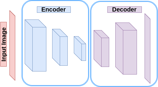
Figure 1: Autoencoder
The MNIST dataset contains vectorized images of 28X28. Therefore we define a new function to reshape each batch of MNIST images to 28X28 and then resize to 32X32. The reason of resizing to 32X32 is to make it a power of two and therefore we can easily use the stride of 2 for downsampling and upsampling.
import numpy as np
from skimage import transform

def resize_batch(imgs):
    # A function to resize a batch of MNIST images to (32, 32)
    # Args:
    #   imgs: a numpy array of size [batch_size, 28 X 28].
    # Returns:
    #   a numpy array of size [batch_size, 32, 32].
    imgs = imgs.reshape((-1, 28, 28, 1))
    resized_imgs = np.zeros((imgs.shape[0], 32, 32, 1))
    for i in range(imgs.shape[0]):
        resized_imgs[i, ..., 0] = transform.resize(imgs[i, ..., 0], (32, 32))
    return resized_imgs
Now we create an autoencoder, define a square error loss and an optimizer.
import tensorflow as tf

ae_inputs = tf.placeholder(tf.float32, (None, 32, 32, 1))  # input to the network (MNIST images)
ae_outputs = autoencoder(ae_inputs)  # create the Autoencoder network

# calculate the loss and optimize the network
loss = tf.reduce_mean(tf.square(ae_outputs - ae_inputs))  # claculate the mean square error loss
train_op = tf.train.AdamOptimizer(learning_rate=lr).minimize(loss)

# initialize the network
init = tf.global_variables_initializer()
Now we can read the batches, train the network and finally test the network by reconstructing a batch of test images.
from tensorflow.examples.tutorials.mnist import input_data

batch_size = 500  # Number of samples in each batch
epoch_num = 5     # Number of epochs to train the network
lr = 0.001        # Learning rate

# read MNIST dataset
mnist = input_data.read_data_sets("MNIST_data", one_hot=True)

# calculate the number of batches per epoch
batch_per_ep = mnist.train.num_examples // batch_size

with tf.Session() as sess:
    sess.run(init)
    for ep in range(epoch_num):  # epochs loop
        for batch_n in range(batch_per_ep):  # batches loop
            batch_img, batch_label = mnist.train.next_batch(batch_size)  # read a batch
            batch_img = batch_img.reshape((-1, 28, 28, 1))               # reshape each sample to an (28, 28) image
            batch_img = resize_batch(batch_img)                          # reshape the images to (32, 32)
            _, c = sess.run([train_op, loss], feed_dict={ae_inputs: batch_img})
            print('Epoch: {} - cost= {:.5f}'.format((ep + 1), c))

    # test the trained network
    batch_img, batch_label = mnist.test.next_batch(50)
    batch_img = resize_batch(batch_img)
    recon_img = sess.run([ae_outputs], feed_dict={ae_inputs: batch_img})[0]

    # plot the reconstructed images and their ground truths (inputs)
    plt.figure(1)
    plt.title('Reconstructed Images')
    for i in range(50):
        plt.subplot(5, 10, i+1)
        plt.imshow(recon_img[i, ..., 0], cmap='gray')
    plt.figure(2)
    plt.title('Input Images')
    for i in range(50):
        plt.subplot(5, 10, i+1)
        plt.imshow(batch_img[i, ..., 0], cmap='gray')
    plt.show()