Convolutional Neural Networks¶

Overview
Motivation
Architecture
Training
Summary
References

Overview ¶

In the last module, we started our dive into deep learning by talking about multi-layer perceptrons. In this module, we will learn about convolutional neural networks also called CNNs or ConvNets. CNNs differ from other neural networks in that sequential layers are not necessarily fully connected. This means that a subset of the input neurons may only feed into a single neuron in the next layer. Another interesting feature of CNNs is their inputs. With other neural networks we might use vectors as inputs, but with CNNs we are typically working with images and other objects with many dimensions. Figure 1 shows some sample images that are each 6 pixels by 6 pixels. The first image is colored and has three channels for red, green, and blue values. The second image is black-and-white and only has one channel for gray values

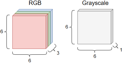
Figure 1. Two sample images and their color channels

Motivation ¶

CNNs are widely used in computer vision where we are trying to analyze visual imagery. CNNs can also be used for other applications such as natural language processing. We will be focusing on the former case here because it is one of the most common applications of CNNs.

Because we assume that we’re working with images, we can design our architecture so that it specifically does a good job at analyzing images. Images have heights, depths, and one or more channels for color. In an image, there might be lines and edges that make up shapes as well as more complex structures such as cars and faces. We will potentially need to identify a large set of relevant features in order to properly classify an image. But just identifying individual features in an image usually isn’t enough. Say we have an image that may or may not be a face. If we saw three noses, an eye, and an ear, we probably wouldn’t call it a face even though those are common features of a face. So then we must also care about where features are located in the image and their proximity to other features. This is a lot of information to keep track of! Fortunately, the architecture of CNNs will cover a lot of these requirements.

Architecture ¶

The architecture of a CNN can be broken down into an input layer, a set of hidden layers, and an output layer. These are shown in Figure 2.

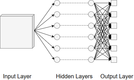
Figure 2. The layers of a CNN

The hidden layers are where the magic happens. The hidden layers will break down our input image in order to identify features present in the image. The initial layers focus on low-level features such as edges while the later layers progressively get more abstract. At the end of all the layers, we have a fully connected layer with neurons for each of our classification values. What we end up with is a probability for each of the classification values. We choose the classification with the highest probability as our guess for what the image show.

Below, we will talk about some types of layers we might use in our hidden layers. Remember that sequential layers are not necessarily fully connected with the exception of the final output layer.

Convolutional Layers ¶

The first type of layer we will discuss is called a convolutional layer. The convolutional description comes from the concept of a convolution in mathematics. Roughly, a convolution is some operation that acts on two input functions and produces an output function that combines the information present in the inputs. The first input will be our image and the second input will be some sort of filter such as a blur or sharpen. When we combine our image with the filter, we extract some information about the image. This process is shown in Figure 3. This is precisely how the CNN will go about extracting features.

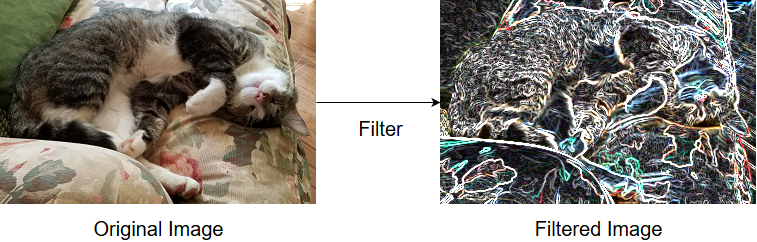
Figure 3. An image before and after filtering

In the human eye, a single neuron is only responsible for a small region of our field of view. It is through many neurons with overlapping regions that we are able to see the world. CNNs are similar. The neurons in a convolutional layer are only responsible for analyzing a small region of the input image but overlap so that we ultimately analyze the whole image. Let’s examine that filter concept we mentioned above.

The filter or kernel is one of the functions used in the convolution. The filter will likely have a smaller height and width than the input image and can be thought of as a window sliding over the image. Figure 4 shows a sample filter and the region of the image it will interact with in the first step of convolution.

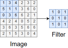
Figure 4. A sample filter and sample window of an image

As the filter moves across the image, we are calculating values for the convolution output called a feature map. At each step, we multiply each entry in the image sample and filter elementwise and sum up all the products. This becomes an entry in the feature map. This process is shown in Figure 5.

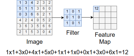
Figure 5. Calculating an entry in the feature map

After the window traverses the entire image, we have the complete feature map. This is shown in Figure 6.

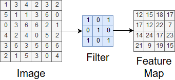
Figure 6. The complete feature map

In the example above, we moved the filter one unit horizontally or one unit vertically from some previous position. This value is called the stride. We could have used other values for the stride but using one everywhere tends to produce the best results.

You may have noticed that the feature map we ended up with had a smaller height and width than the original image sample. This is a result of the way we moved the filter around the sample. If we wanted the feature map to have the same height and width, we could pad the sample. This involves adding zero entries around the sample so that moving the filter keeps the dimensions of the original sample in the feature map. Figure 7 illustrates this process.

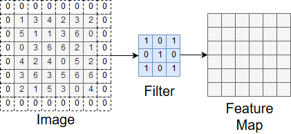
Figure 7. Padding before applying a filter

A feature map represents one type of feature we’re analyzing the image for. Often, we want to analyze the image for a bunch of features so we end up with a bunch of feature maps! The output of the convolution layer is a set of feature maps. Figure 8 shows the process of going from an image to the resulting feature maps.

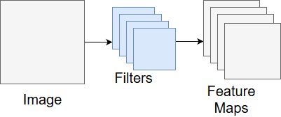
Figure 8. The output of a convolutional layer

After a convolutional layer, it is common to have a ReLU (rectified linear unit) layer. The purpose of this layer is to introduce non-linearity into the system. Basically, real-world problems are rarely nice and linear so we want our CNN to account for this when it trains. A good explanation of this layer requires math that we don’t expect you to know. If you are curious about the topic, you can find an explanation here.

Pooling Layers ¶

The next type of layer we will cover is called a pooling layer. The purpose of pooling layers are to reduce the spatial size of the problem. This in turn reduces the number of parameters needed for processing and the total amount of computation in the CNN. There are several options for pooling but we will cover the most common approach, max pooling.

In max pooling, we slide a window over the input and take the max value in the window at each step. This process is shown in Figure 9.

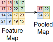
Figure 9. Max pooling on a feature map

Max pooling is good because it maintains important features about the input, reduces noise by ignoring small values, and reduces the spatial size of the problem. We can use these after convolutional layers to keep the computation of problems manageable.

Fully Connected Layers ¶

The last type of layer we will discuss is called a fully connected layer. Fully connected layers are used to make the final classification in the CNN. They work exactly like they do in other neural networks. Before moving to the first fully connected layer, we must flatten our input values into a one-dimensional vector that the layer can interpret. Figure 10 shows a simple example of converting a multi-dimensional input into a one-dimensional vector.

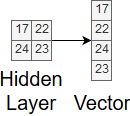
Figure 10. Flattening input values

After doing this, we may have several fully connected layers before the final output layer. The output layer uses some function, such as softmax, to convert the neuron values into a probability distribution over our classes. This means that the image has a certain probability for being classified as one of our classes and the sum of all those probabilities equals one. This is clearly visible in Figure 11.

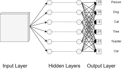
Figure 11. The final probabilistic outputs

Training ¶

Now that we have the architecture in place for CNNs we can move on to training. Training a CNN is pretty much exactly the same as training a normal neural network. There is some added complexity due to the convolutional layers but the strategies for training remain the same. Techniques, such as gradient descent or backpropagation, can be used to train filter values and other parameters in the network. As with all the other training we have covered, having a large training set will improve the performance of the CNN. The problem with training CNNs and other deep learning models is that they are much more complex than the models we covered in earlier modules. This results in training being much more computationally expensive to the point where we would need specialized hardware like GPUs to run our code. However, we get what we pay for because deep learning models are much more powerful than the models covered in earlier modules.

Summary ¶

In this module, we learned about convolutional neural networks. CNNs differ from other neural networks because they usually take images as input and can have hidden layers that are not fully connected. CNNs are powerful tools widely used in image classification applications. By using a variety of hidden layers, we can extract features from an image and use them to probabilistically guess a classification. CNNs are also complex models and understanding how they work can be an intimidating task. We hope that the information presented gives you a better understanding of how CNNs work so that you can continue to learn about them and deep learning.