Clustering¶

Overview
Clustering
Motivation
Methods
- K-Means
- Hierarchical
Summary
References

Overview ¶

In previous modules, we talked about supervised learning topics. We are now ready to move on to unsupervised learning where our goals will be much different. In supervised learning, we tried to match inputs to some existing patterns. For unsupervised learning, we will try to discover patterns in raw, unlabeled data sets. We saw classification problems come up often in supervised learning and we will now examine a similar problem in unsupervised learning: clustering.

Clustering ¶

Clustering is the process of grouping similar data and isolating dissimilar data. We want the data points in clusters we come up with to share some common properties that separate them from data points in other clusters. Ultimately, we’ll end up with a number of groups that meet these requirements. This probably sounds familiar because on the surface it sounds a lot like classification. But be aware that clustering and classification solve two very different problems. Clustering is used to identify potential groups in a data set while classification is used to match an input to an existing group.

Motivation ¶

Clustering is a very useful technique for solving problems that commonly arise in unsupervised learning. With clustering, we can find underlying patterns in a data set by grouping similar data points. Consider the case of a toy manufacturer. The toy manufacturer makes a lot of products and happens to have a diverse consumer base. It could be useful for the manufacturer to identify groups that buy particular products so it can personalize advertisements. Targeted advertising is a common desire in marketing and clustering helps identify demographics. When we want to identify potential group structures in a raw data set, clustering is a good tool to use.

Methods ¶

Because clustering just provides an interpretation of a data set, there are many ways to go about implementing it. We might consider the distance between data points when deciding on clusters. We could also consider how dense data points are in a region to determine clusters. For this module, we will analyze two of the more common and popular methods: K-Means and Hierarchical. In both cases, we will use the data set in Figure 1 for analysis.

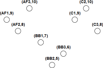
Figure 1. A data set to use for clustering

This data set represents product data for a toy manufacturer. The manufacturer sells 3 products with 3 variants each to young children between the ages of 5 and 10. These products are action figures, building blocks, and cars. The manufacturer has also noted which age group buys the most of each product. Each point in the data set represents one of the toys and the age group that buys the most of them.

K-Means ¶

K-Means clustering attempts to divide a data set into K clusters using an iterative process. The first step is choosing a center point for each cluster. This center point does not need to correspond to an actual data point. The center points could be chosen at random or we could pick them if we have a good guess of where they should be. In the code below, the center points are chosen using the k-means++ method which is designed to speed up convergence. Analysis of this method is beyond the scope of this module but for additional initial options in sklearn, check here.

The second step is assigning each data point to a cluster. We do this by measuring the distance between a data point and each center point and choosing the cluster whose center point is the closest. This step is illustrated in Figure 2.

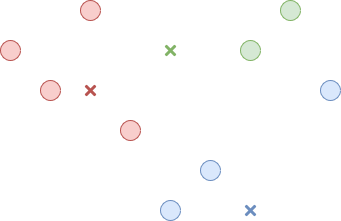
Figure 2. Associate each point with a cluster

Now that all the data points belong to a cluster, the third step is recomputing the center point of each cluster. This is just the average of all the data points belonging to the cluster. This step is illustrated in Figure 3.

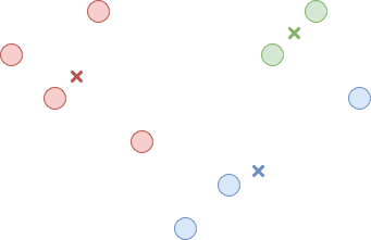
Figure 3. Find the new center for each cluster

Now we just repeat the second and third step until the centers stop changing or only change slightly between iterations. The result is K clusters where data points are closer to their cluster’s center than any other cluster’s center. This is illustrated in Figure 4.

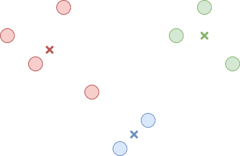
Figure 4. The final clusters

K-Means clustering requires us to input the number of expected clusters which isn’t always easy to determine. It can also be inconsistent depending on where we choose the starting center points in the first step. Over the course of the process, we may end up with clusters that appear to be optimized but may not be the best overall solution. In Figure 4, we end with a red data point that is equally far from the red center and the blue center. This stemmed from our initial center choices. In contrast, Figure 5 shows another result we may have reached given different starting centers and looks a little better.

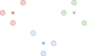
Figure 5. An alternative set of clusters

On the other hand, K-Means is very powerful because it considers the entire data set at each step. It is also fast because we’re only ever computing distances. So if we want a fast technique that considers the whole data set and we have some knowledge of what the underlying groups might look like, K-Means is a good choice.

The relevant code is available in the clustering_kmeans.py file.

In the code, we create the simple data set to use for analysis. Setting up the clustering is very simple and requires one line of code:

kmeans = KMeans(n_clusters=3, random_state=0).fit(x)

The n_clusters parameter was chosen to be 3 because there appears to be 3 clusters in out data set. The random_state parameter is just there to give a consistent result each time you run the code. The rest of the code is to display the final plot shown in Figure 6.

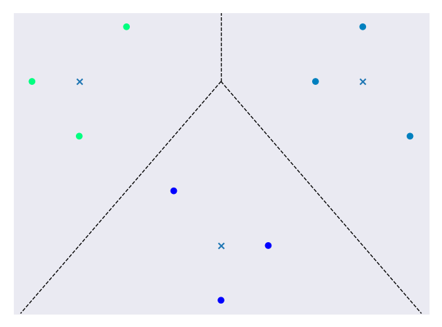
Figure 6. A final clustered data set

The clusters are color coded, the ‘x’s represent cluster centers, and the dotted lines represent cluster boundaries.

Hierarchical ¶

Hierarchical clustering imagines the data set as a hierarchy of clusters. We could start by making one giant cluster out of all the data points. This is illustrated in Figure 7.

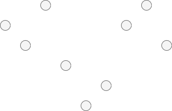
Figure 7. One giant cluster in the data set*

Inside of this cluster, we find the two least similar sub-clusters and split them. This can be done by using an algorithm to maximize the inter-cluster distance. This is just the smallest distance between a node from one cluster and a node from the other cluster. This is illustrated in Figure 8.

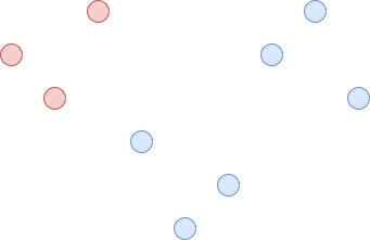
Figure 8. The giant cluster is split into 2 clusters

We continue to split the sub-clusters until every data point belongs to its own cluster or until we decide to stop. If we start from one giant cluster and break it down into successively smaller clusters, it is called top-down or divisive clustering. Alternatively, we could start by considering a cluster for every data point. The next step would be to combine the two closest clusters into a larger cluster. This can be done by finding the distance between every cluster and choosing the pair with the least distance between them. We would continue this process until we had a single cluster. This method of combining clusters is called bottom-up or agglomerative clustering. At any point in these two methods, we can stop when the clusters look appropriate.

Unlike K-Means, Hierarchical clustering is relatively slow so it doesn’t scale as well to large data sets. On the bright side, Hierarchical clustering is more consistent when you run it multiple times and doesn’t require you to know the number of expected clusters.

The relevant code is available in the clustering_hierarchical.py file.

In the code, we create the simple data set to use for analysis. Setting up the clustering is very simple and requires one line of code:

hierarchical = AgglomerativeClustering(n_clusters=3).fit(x)

The n_clusters parameter was chosen to be 3 because there appears to be 3 clusters in out data set. If we didn’t already know this, we could try out different values and see which one worked the best. The rest of the code is to display the final plot shown in Figure 9.

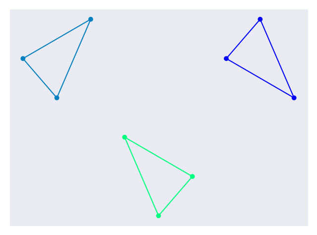
Figure 9. A final clustered data set

The clusters are color coded and large clusters are surrounded with a border to show which data points belong to them.

Summary ¶

In this module, we learned about clustering. Clustering allows us to discover patterns in a raw data set by grouping similar data points. This is a common desire in unsupervised learning and clustering is a popular technique. You may have noticed that the methods discussed above were relatively simple compared to some of the more math-heavy descriptions in previous modules. These methods are simple but powerful. For example, we were able to determine clusters in the toy manufacturer example that could be used for targeted advertising. This is a very useful result for businesses and it only took us a few lines of code. By developing a good understanding of clustering, you are setting yourself up for success in the machine learning world.