Decision Trees¶

Introduction
Motivation
Classification and Regression Trees
Splitting (Induction)
Cost of Splitting
Pruning
Conclusion
Code Example
References

Introduction ¶

Decision trees are a classifier in machine learning that allows us to make predictions based on previous data. They are like a series of sequential “if … then” statements you feed new data into to get a result.

To demonstrate decision trees, let’s take a look at an example. Imagine we want to predict whether Mike is going to go grocery shopping on any given day. We can look at previous factors that led Mike to go to the store:

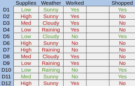
Figure 1. An example dataset

Here we can see the amount of grocery supplies Mike had, the weather, and whether Mike worked each day. Green rows are days he went to the store, and red days are those he didn’t. The goal of a decision tree is to try to understand why Mike goes to the store, and apply that to new data later on.

Let’s divide the first attribute up into a tree. Mike can either have a low, medium, or high amount of supplies:

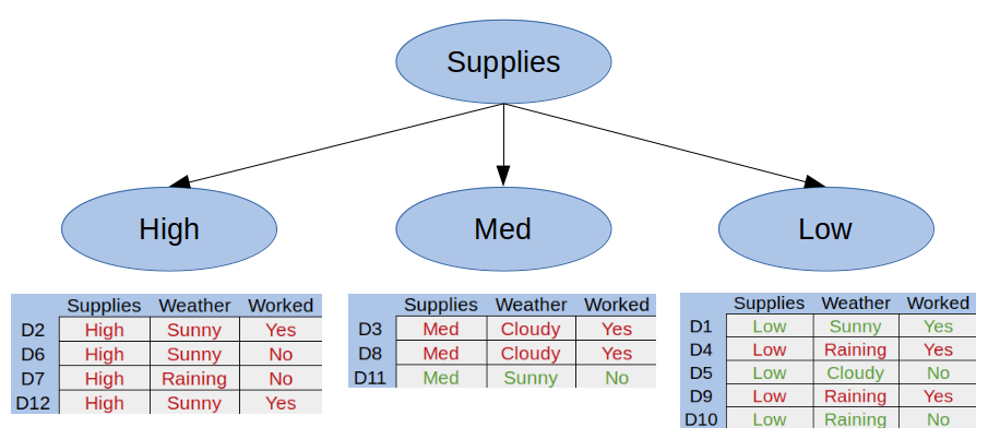
Figure 2. Our first split

Here we can see that Mike never goes to the store if he has a high amount of supplies. This is called a pure subset, a subset with only positive or only negative examples. With decision trees, there is no need to break a pure subset down further.

Let’s break the Med Supplies category into whether Mike worked that day:

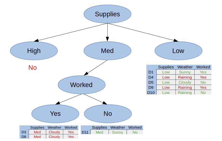
Figure 3. Our second split

Here we can see we have two more pure subsets, so this tree is complete. We can replace any pure subsets with their respective answer - in this case, yes or no.

Finally, let’s split the Low Supplies category by the Weather attribute:

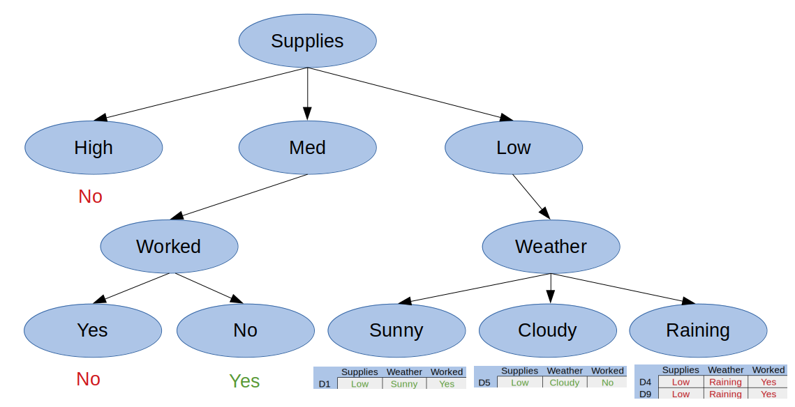
Figure 4. Our third split

Now that we have all pure subsets, we can create our final decision tree:

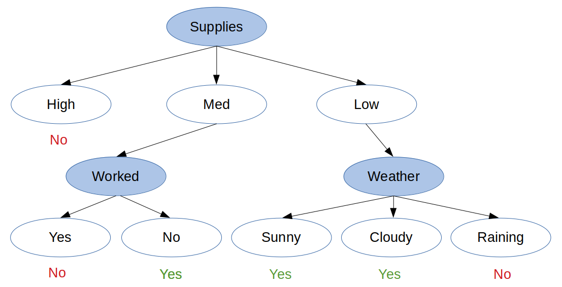
Figure 5. The final decision tree

Motivation ¶

Decision trees are easily created, visualized, and interpreted. Because of this, they are typically the first method used to model a dataset. The hierarchical structure and categorical nature of a decision tree makes it highly intuitive to implement. Decision trees expand logarithmically based on the number of data points you have, meaning larger datasets will impact the tree creation process less than other classifiers. Because of the tree structure, classifying new data points is also performed logarithmically.

Classification and Regression Trees ¶

Decision tree algorithms are also known as CART, or Classification and Regression Trees. A Classification Tree, like the one shown above, is used to get a result from a set of possible values. A Regression Tree is a decision tree where the result is a continuous value, such as the price of a car.

Splitting (Induction)¶

Decision trees are created through a process of splitting called induction, but how do we know when to split? We need a recursive algorithm that determines the best attributes to split on. One such algorithm is the greedy algorithm:

Starting from the root, we create a split for each attribute.
For each created split, calculate the cost of the split.
Choose the split that costs the least.
Recurse into the sub-trees and continue from step 1.

This process is repeated until all nodes have the same value as the target result, or splitting adds no value to a prediction. This algorithm has the root node as the best classifier.

Cost of Splitting ¶

The cost of a split is determined by a cost function. The goal of using a cost function is to split the data in a way that can be computed and that provides the most information gain.

For classification trees, those that provide an answer rather than a value, we can compute imformation gain using Gini Impurities:

Equation 1. The Gini Impurity Function

Ref: https://sebastianraschka.com/faq/docs/decision-tree-binary.html

Equation 2. The Gini Information Gain Formula

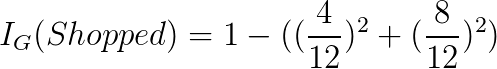
Ref: https://sebastianraschka.com/faq/docs/decision-tree-binary.html

To calculate information gain, we first start by computing the Gini Impurity of our root node. Let’s take a look at the data we used earlier:

	Supplies	Weather	Worked?	Shopped?
D1	Low	Sunny	Yes	Yes
D2	High	Sunny	Yes	No
D3	Med	Cloudy	Yes	No
D4	Low	Raining	Yes	No
D5	Low	Cloudy	No	Yes
D6	High	Sunny	No	No
D7	High	Raining	No	No
D8	Med	Cloudy	Yes	No
D9	Low	Raining	Yes	No
D10	Low	Raining	No	Yes
D11	Med	Sunny	No	Yes
D12	High	Sunny	Yes	No

Our root node is the target variable, whether Mike is going to go shopping. To calculate its Gini Impurity, we need to find the sum of probabilities squared for each outcome and subtract this result from one:

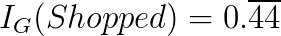
Let’s calculate the Gini Information Gain if we split on the first attribute, Supplies. We have three different categories we can split by - Low, Med, and High. For each of these, we calculate its Gini Impurity:

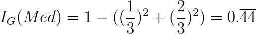
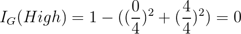
As you can see, the impurity for High supplies is 0. This means that if we split on Supplies and receive High input, we immediately know what the outcome will be. To determine the Gini Information Gain for this split, we compute the root’s impurity minus the weighted average of each child’s impurity:

We continue this pattern for every possible split, then choose the split that gives us the highest information gain value. Maximizing information gain leaves us with the most polarized splits possible, lowering the probability new input is incorrectly classified.

Pruning ¶

A decision tree created through a sufficiently large dataset may end up with an excessive amount of splits, each with decreasing usefulness. A highly detailed decision tree can even lead to overfitting, discussed in the previous module. Because of this, it’s beneficial to prune less important splits of a decision tree away. Pruning involves calculating the information gain of each ending sub-tree (the leaf nodes and their parent node), then removing the sub-tree with the least information gain:

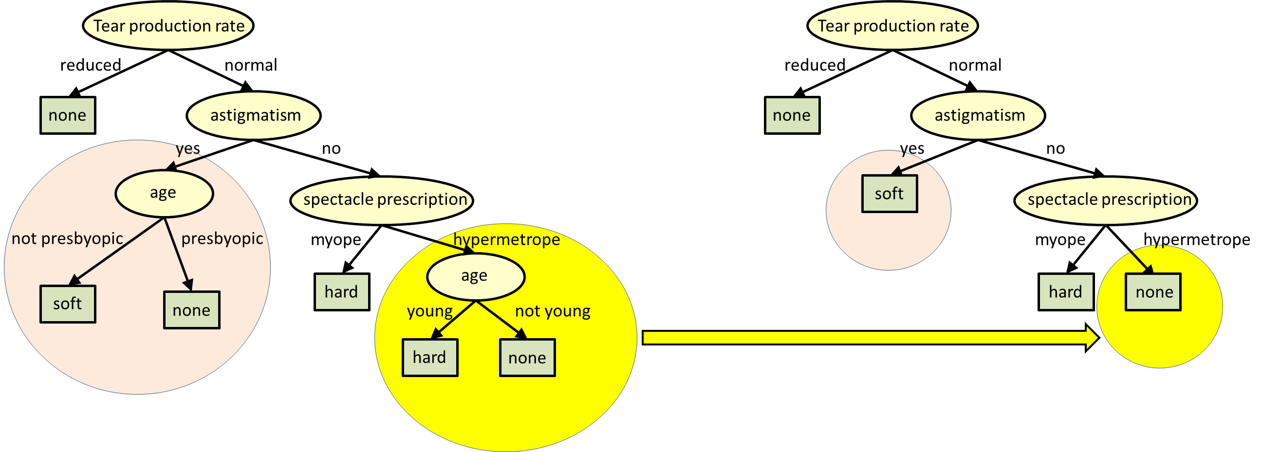
Ref: http://www.cs.cmu.edu/~bhiksha/courses/10-601/decisiontrees/

As you can see, the sub-tree is replaced with the more prominent result, becoming a new leaf. This process can be repeated until you reach a desired complexity level, tree height, or information gain amount. Information gain can be tracked and stored as the tree is built to save time when pruning as well. Each model should make use of its own pruning algorithm to meet its needs.

Conclusion ¶

Decision trees allow you to quickly and efficiently classify data. Because they shape data into a heirarchy of decisions, they are highly understandable by even non-experts. Decision trees are created and refined in a two-step process - induction and pruning. Induction involves picking the best attribute to split on, while pruning helps to filter out results deemed useless. Because decision trees are so simple to create and understand, they are typically the first approach used to model and predict outcomes of a dataset.

Code Example ¶

The provided code, decisiontrees.py takes the example discussed in this documentation and creates a decision tree from it. First, each possible option for each class is defined. This is used later to fit and display our decision tree:

# The possible values for each class
classes = {
    'supplies': ['low', 'med', 'high'],
    'weather':  ['raining', 'cloudy', 'sunny'],
    'worked?':  ['yes', 'no']
}

Next, we’ve created a matrix of the dataset shown above and defined each row’s outcome:

# Our example data from the documentation
data = [
    ['low',  'sunny',   'yes'],
    ['high', 'sunny',   'yes'],
    ['med',  'cloudy',  'yes'],
    ['low',  'raining', 'yes'],
    ['low',  'cloudy',  'no' ],
    ['high', 'sunny',   'no' ],
    ['high', 'raining', 'no' ],
    ['med',  'cloudy',  'yes'],
    ['low',  'raining', 'yes'],
    ['low',  'raining', 'no' ],
    ['med',  'sunny',   'no' ],
    ['high', 'sunny',   'yes']
]

# Our target variable, whether someone went shopping
target = ['yes', 'no', 'no', 'no', 'yes', 'no', 'no', 'no', 'no', 'yes', 'yes', 'no']

Unfortunately, the sklearn machine learning package can’t create a decision tree from categorical data. There is in-progress work to allow this, but for now we need another way to represent the data in a decision tree with the library. A naive approach would be to just enumerate each category - for instance, converting sunny/raining/cloudy to values such as 0, 1, and 2. There are some unfortunate side effects of doing this though, such as the values being comparable (sunny < raining) and continuous. To get around this, we “one hot encode” the data:

categories = [classes['supplies'], classes['weather'], classes['worked?']]
encoder = OneHotEncoder(categories=categories)

x_data = encoder.fit_transform(data)

One hot encoding allows us to convert categorical data into values recognizable by ML algorithms expecting continuous data. It works by taking a class and dividing it up into each option, with a bit representing whether the option is present.

Now that we have data suited to sklearn’s decision tree model, we simply fit the classifier to the data:

# Form and fit our decision tree to the now-encoded data
classifier = DecisionTreeClassifier()
tree = classifier.fit(x_data, target)

The rest of the code involves creating some random prediction input to show how you can use the tree. We create a random set of data in the same format as the data above, then pass it into DecisionTreeClassifier’s predict method. This gives us an array of predicted target variables - in this case, yes or no answers to whether Mike will go shopping:

# Use our tree to predict the outcome of the random values
prediction_results = tree.predict(encoder.transform(prediction_data))