Regularization
Motivation
Consider the following scenario. You are making a peanut butter sandwich and are trying to adjust ingredients so that it has the best taste. You might consider the type of bread, type of peanut butter, or peanut butter to bread ratio in your decision making process. But would you consider other factors like how warm it is in the room, what you had for breakfast, or what color socks you’re wearing? You probably wouldn’t as these things don’t have as much impact on the taste of your sandwich. You would focus more on the first few features for whatever recipe you end up using and avoid paying too much attention to the other ones. This is the basic idea of regularization.
Overview
In previous modules, we have seen prediction models trained on some sample set and scored against how close they are to a test set. We obviously want our models to make predictions that are accurate but can they be too accurate? When we look at a set of data, there are two main components: the underlying pattern and noise. We only want to match the pattern and not the noise. Consider the figures below that represent quadratic data. Figure 1 uses a linear model to approximate the data. Figure 2 uses a quadratic model to approximate the data. Figure 3 uses a high degree polynomial model to approximate the data.
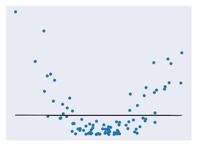
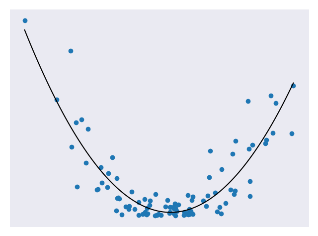
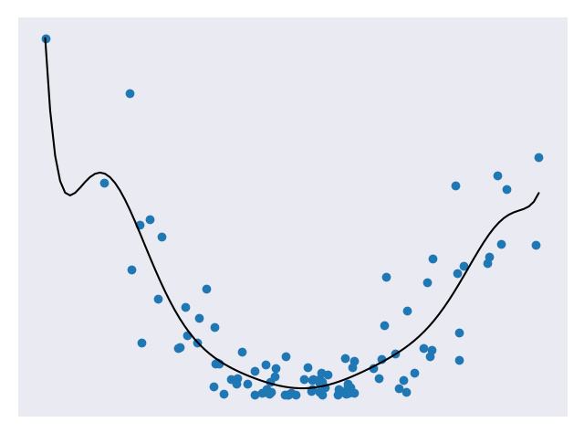
Figure 1 underfits the data, Figure 2 looks to be a pretty good fit for the data, and Figure 3 is a very close fit for the data. Of all the models above, the third is likely the most accurate for the test set. But this isn’t necessarily a good thing. If we add in some more test points, we’ll likely find that the third model is no longer as accurate at predicting them but the second model is still pretty good. This is because the third model suffers from overfitting. Overfitting means it does a really good job at fitting the test data (including noise) but is bad at generalizing to new data. The second model is a nice fit for the data and is not so complex that it won’t generalize.
The goal of regularization is to avoid overfitting by penalizing more complex models. The general form of regularization involves adding an extra term to our cost function. So if we were using a cost function CF, regularization might lead us to change it to CF + λ * R where R is some function of our weights and λ is a tuning parameter. The result is that models with higher weights (more complex) get penalized more. The tuning parameter basically lets us adjust the regularization to get better results. The higher the λ the less impact the weights have on the total cost.
Methods
There are many methods we can use for regularization. Below we’ll cover some of the more common ones and when they are good to use.
Ridge Regression
Ridge regression is a type of regularization where the function R involves summing the squares of our weights. Equation 1 shows an example of the modified cost function.
Equation 1. A cost function for ridge regression
Equation 1 is an example of the regularization with w representing our weights. Ridge regression forces weights to approach zero but will never cause them to be zero. This means that all the features will be represented in our model but overfitting will be minimized. Ridge regression is a good choice when we don’t have a very large number of features and just want to avoid overfitting. Figure 4 gives a comparison of a model with and without ridge regression applied.
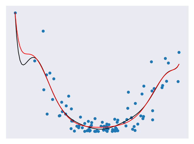
In Figure 4, the black line represents a model without Ridge regression applied and the red line represents a model with Ridge regression applied. Note how much smoother the red line is. It will probably do a better job against future data.
In the included regularization_ridge.py file, the code that adds ridge regression is:
Adding the Ridge regression is as simple as adding an additional argument to our Pipeline call. Here, the parameter alpha represents our tuning variable. For additional information on Ridge regression in scikit-learn, consult here.
Lasso Regression
Lasso regression is a type of regularization where the function R involves summing the absolute values of our weights. Equation 2 shows an example of the modified cost function.
Equation 2. A cost function for lasso regression
Equation 2 is an example of the regularization with w representing our weights. Notice how similar ridge regression and lasso regression are. The only noticeable difference is that square on the weights. This happens to have a big impact on what they do. Unlike ridge regression, lasso regression can force weights to be zero. This means that our resulting model may not even consider some of the features! In the case we have a million features where only a small amount are important, this is an incredibly useful result. Lasso regression lets us avoid overfitting and focus on a small subset of all our features. In the original scenario, we would end up ignoring those factors that don’t have as much impact on our sandwich eating experience. Figure 5 gives a comparison of a model with and without lasso regression applied.
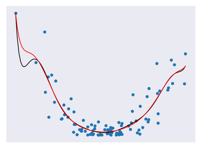
In the figure above, the black line represents a model without Lasso regression applied and the red line represents a model with Lasso regression applied. The red line is much smoother than the black line. The Lasso regression was applied to a model of degree 10 but the result looks like it has a much lower degree! The Lasso model will probably do a better job against future data.
In the included regularization_lasso.py file, the code that adds Lasso regression is:
Adding the Lasso regression is as simple as adding the Ridge regression. Here,
the parameter alpha represents our tuning variable and max_iter represents
the max number of iterations to run for. For additional information on Lasso
regression in scikit-learn, consult here.
Summary
In this module, we learned about regularization. With regularization, we have found a good way to avoid overfitting our data. This is a common but important problem in modeling so it’s good to know how to mediate it. We have also explored some methods of regularization that we can use in different situations. With this, we have learned enough about the core concepts of machine learning to move onto our next major topic, supervised learning.
References
- https://towardsdatascience.com/regularization-in-machine-learning-76441ddcf99a
- https://www.analyticsvidhya.com/blog/2018/04/fundamentals-deep-learning-regularization-techniques
- https://www.quora.com/What-is-regularization-in-machine-learning
- https://scikit-learn.org/stable/modules/generated/sklearn.linear_model.Ridge.html
- https://scikit-learn.org/stable/modules/generated/sklearn.linear_model.Lasso.html