Naive Bayes Classification
Motivation
A recurring problem in machine learning is the need to classify input into some preexisting class. Consider the following example.
Say we want to classify a random piece of fruit we found lying around. In this example, we have three existing fruit categories: apple, blueberry, and coconut. Each of these fruits have three features we care about: size, weight, and color. This information is shown in Figure 1.
| Apple | Blueberry | Coconut | |
|---|---|---|---|
| Size | Moderate | Small | Large |
| Weight | Moderate | Light | Heavy |
| Color | Red | Blue | Brown |
We observe the piece of fruit we found and determine it has a moderate size, it is heavy, and it is red. We can compare these features against the features of our known classes to guess what type of fruit it is. The unknown fruit is heavy like a coconut but it shares more features with the apple class. The unknown fruit shares 2 of 3 characteristics with the apple class so we guess that it’s an apple. We used the fact that the random fruit is moderately sized and red like an apple to make our guess.
This example is a bit silly but it highlights some fundamental points about classification problems. In these types of problems, we are comparing features of an unknown input to features of known classes in our data set. Naive Bayes classification is one way to do this.
What is it?
Naive Bayes is a classification technique that uses probabilities we already know to determine how to classify input. These probabilities are related to existing classes and what features they have. In the example above, we choose the class that most resembles our input as its classification. This technique is based around using Bayes’ Theorem. If you’re unfamiliar with what Bayes’ Theorem is, don’t worry! We will explain it in the next section.
Bayes’ Theorem
Bayes’ Theorem [Equation 1] is a very useful result that shows up in probability theory and other disciplines.
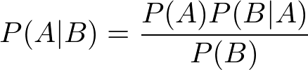
Equation 1. Bayes’ Theorem
With Bayes’ Theorem, we can examine conditional probabilities (the probability of an event happening given another event has happened). P(A|B) is the probability that event A will happen given that event B has already happened. We can determine this value using other information we know about events A and B. We need to know P(B|A) (the probability that event B will happen given that event A has already happened), P(B) (the probability event B will happen), and P(A) (the probability event A will happen). We can even apply Bayes’ Theorem to machine learning problems!
Naive Bayes
Naive Bayes classification uses Bayes’ Theorem with some additional assumptions. The main thing we will assume is that features are independent. Assuming independence means that the probability of a set of features occurring given a certain class is the same as the product of all the probabilities of each individual feature occurring given that class. In the case of our fruit example above, being red does not affect the probability of being moderately sized so assuming independence between color and size is fine. This is often not the case in real-world problems where features may have complex relationships. This is why “naive” is in the name. If the math seems complicated, don’t worry! The code will handle the number crunching for us. Just remember that we are assuming that features are independent of each other to simplify calculations.
In this technique, we take some input and calculate the probability of it happening given that it belongs to one of our classes. We must do this for each of our classes. After we have all these probabilities, we just take the one that’s the largest as our prediction for what class the input belongs to.
Algorithms
Below are some common models used for Naive Bayes classification. We have separated them into two general cases based on what type of feature distributions they use: continuous or discrete. Continuous means real-valued (you can have decimal answers) and discrete means a count (you can only have whole number answers). Also provided are the relevant code snippets for each algorithm.
Gaussian Model (Continuous)
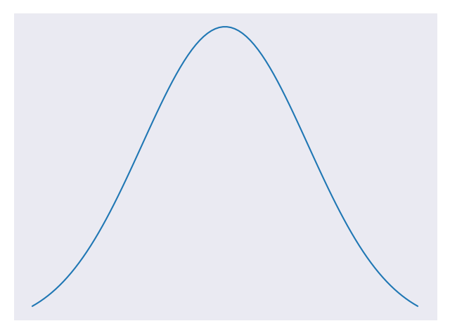
Gaussian models assume features follow a normal distribution. As far as you need to know, a normal distribution is just a specific type of probability distribution where values tend to be close to the average. As you can see in Figure 2, the plot of a normal distribution has a bell shape. Values are most frequent around the peak of the plot and tend to be rarer the farther away you go. This is another big assumption because many features do not follow a normal distribution. While this is true, assuming a normal distribution makes our calculations a whole lot easier. We use Gaussian models when features are not counts and include decimal values.
The relevant code is available in the gaussian.py file.
In the code, we try and guess a color from given RGB percentages. We create some data to work with where each data point represents an RGB triple. The values of the triples are decimals ranging from 0 to 1 and each has a color class it is associated with. We create a Gaussian model and fit it to the data. We then make a prediction with new input to see which color it should be classified as.
Multinomial Model (Discrete)
Multinomial models are used when we are working with discrete counts. Specifically, we want to use them when we are counting how often a feature occurs. For example, we might want to count how often the word “count” appears on this page. Figure 3 shows the sort of data we might use with a multinomial model. If we know the counts will only be one of two values, we should use a Bernoulli model instead.
| Word | Frequency |
|---|---|
| Algebra | 0 |
| Big | 1 |
| Count | 2 |
| Data | 12 |
The relevant code is available in the multinomial.py file.
The code is based on our fruit example. In the code, we try and guess a fruit from given characteristics. We create some data to work with where each data point is a triple representing characteristics of a fruit namely size, weight, and color. The values of the triples are integers ranging from 0 to 2 and each has a fruit class it is associated with. The integers are basically just labels associated with characteristics but using them instead of strings allows us to use a Multinomial model. We create a Multinomial model and fit it to the data. We then make a prediction with new input to see which fruit it should be classified as.
Bernoulli Model (Discrete)
Bernoulli models are also used when we are working with discrete counts. Unlike the multinomial case, here we are counting whether or not a feature occurred. For example, we might want to check if the word “count” appears at all on this page. We can also use Bernoulli models when features only have 2 possible values like red or blue. Figure 4 shows the sort of data we might use with a Bernoulli model.
| Word | Present? |
|---|---|
| Algebra | False |
| Big | True |
| Count | True |
| Data | True |
The relevant code is available in the bernoulli.py file.
In the code, we try and guess if something is a duck or not based on certain characteristics it has. We create some data to work with where each data point is a triple representing the characteristics: walks like a duck, talks like a duck, and is small. The values of the triples are either 1 or 0 for true or false and each is either a duck or not a duck. We create a Bernoulli model and fit it to the data. We then make a prediction with new input to see whether or not it is a duck.
Conclusion
In this module, we learned about Naive Bayes classification. Naive Bayes classification lets us classify an input based on probabilities of existing classes and features. As demonstrated in the code, you don’t need a lot of training data for Naive Bayes to be useful. Another bonus is speed which can come in handy for real-time predictions. We make a lot of assumptions to use Naive Bayes so results should be taken with a grain of salt. But if you don’t have much data and need fast results, Naive Bayes is a good choice for classification problems.
References
- https://machinelearningmastery.com/naive-bayes-classifier-scratch-python/
- https://www.analyticsvidhya.com/blog/2017/09/naive-bayes-explained/
- https://towardsdatascience.com/naive-bayes-in-machine-learning-f49cc8f831b4
- https://medium.com/machine-learning-101/chapter-1-supervised-learning-and-naive-bayes-classification-part-1-theory-8b9e361897d5