Principal Component Analysis
Introduction
Principal component analysis is one technique used to take a large list of interconnected variables and choose the ones that best suit a model. This process of focusing in on only a few variables is called dimensionality reduction, and helps reduce complexity of our dataset. At its root, principal component analysis summarizes data.
Motivation
Principal component analysis is extremely useful for deriving an overall, linearly independent, trend for a given dataset with many variables. It allows you to extract important relationships out of variables that may or may not be related. Another application of principal component analysis is for display - instead of representing a number of different variables, you can create principal components for just a few and plot them.
Dimensionality Reduction
There are two types of dimensionality reduction: feature elimination and feature extraction.
Feature elimination simply involves pruning features from a dataset we deem unnecessary. A downside of feature elimination is that we lose any potential information gained from the dropped features.
Feature extraction, however, creates new variables by combining existing features. At the cost of some simplicity or interpretability, feature extraction allows you to maintain all important information held within features.
Principal component analysis deals with feature extraction (rather than elimination) by creating a set of independent variables called principal components.
PCA Example
Principal component analysis is performed by considering all of our variables and calculating a set of direction and magnitude pairs (vectors) to represent them. For example, let’s consider a small example dataset plotted below:
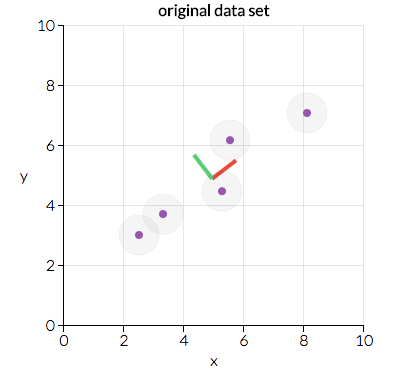
Here we can see two direction pairs, represented by the red and green lines. In this scenario, the red line has a greater magnitude as the points are more clustered across a greater distance than with the green direction. Principal component analysis will use the vector with the greater magnitude to transform the data into a smaller feature space, reducing dimensionality. For example, the above graph would be transformed into the following:
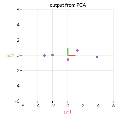
By transforming our data in this way, we’ve ignored a feature that is less important to our model - that is, higher variation along the green dimension will have a greater impact on our results than variation along the red.
The mathematics behind principal component analysis are left out of this discussion for brevity, but if you’re interested in learning about them we highly recommend visiting the references listed at the bottom of this page.
Number of Components
In the example above, we took a two-dimensional feature space and reduced it to a single dimension. In most scenarios though, you will be working with far more than two variables. Principal component analysis can be used to just remove a single feature, but it is often useful to reduce several. There are several strategies you can employ to decide how many feature reductions to perform:
Arbitrarily
This simply involves picking a number of features to keep for your given model. This method is highly dependent on your dataset and what you want to convey. For instance, it may be beneficial to represent your higher-order data on a 2D space for visualization. In this case, you would perform feature reduction until you have two features.
Percent of cumulative variability
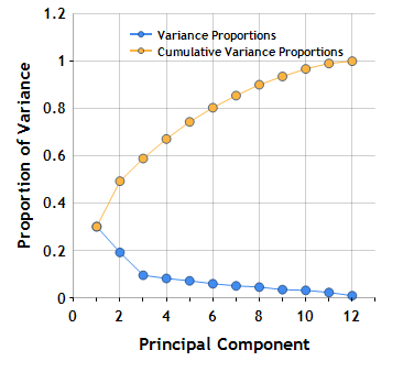
Part of the principal component analysis calculation involves finding a proportion of variance which approaches 1 through each round of PCA performed. This method of choosing the number of feature reduction steps involves selecting a target variance percentage. For instance, let’s look at a graph of cumulative variance at each level of PCA for a theoretical dataset:
The above image is called a scree plot, and is a representation of the cumulative and current proportion of variance for each principal component. If we wanted at least 80% cumulative variance, we would use at least 6 principal components based on this scree plot. Aiming for 100% variance is not generally recommended, as reaching this means your dataset has redundant data.
Percent of individual variability
Instead of using principal components until we reach a cumulative percent of variability, we can instead use principal components until a new component wouldn’t add much variability. In the plot above, we might choose to use 3 principal components since the next components don’t have as strong a drop in variability.
Conclusion
Principal component analysis is a technique to summarize data, and is highly flexible depending on your use case. It can be valuable in both displaying and analyzing a large number of possibly dependent variables. Techniques of performing principal component analysis range from arbitrarily selecting principal components, to automatically finding them until a variance is reached.
Code Example
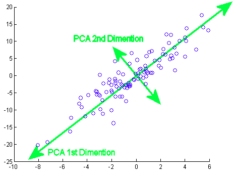
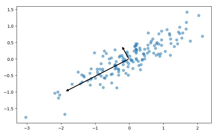
Our example code, pca.py, shows you how to perform principal component analysis on a dataset of random x, y pairs. The script goes through a short process of generating this data, then calls sklearn’s PCA module:
# Find two principal components from our given dataset
pca = PCA(n_components = 2)
pca.fit(points)
Each step in the process includes helpful visualizations using matplotlib. For instance, the principal components fitted above are plotted as two vectors on the dataset:
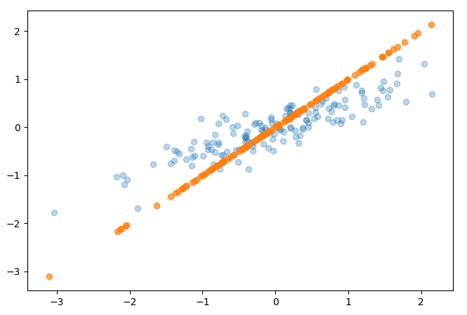
The script also shows how to perform dimensionality reduction, discussed above. In sklearn, this is done by simply calling the transform method once a PCA is fitted, or doing both steps at the same time with fit_transform:
# Reduce the dimensionality of our data using a PCA transformation
pca = PCA(n_components = 1)
transformed_points = pca.fit_transform(points)
The end result of our transformation is just a series of X values, though the code example performs an inverse transformation for plotting the result in the following graph:
References
- http://www.cs.otago.ac.nz/cosc453/student_tutorials/principal_components.pdf
- https://towardsdatascience.com/a-one-stop-shop-for-principal-component-analysis-5582fb7e0a9c
- https://towardsdatascience.com/pca-using-python-scikit-learn-e653f8989e60
- https://en.wikipedia.org/wiki/Principal_component_analysis
- https://stats.stackexchange.com/questions/2691/making-sense-of-principal-component-analysis-eigenvectors-eigenvalues
- https://www.centerspace.net/clustering-analysis-part-i-principal-component-analysis-pca